PyDAQviewer Tutorial

Ahmed Ammar [1, 2] (ahmed.ammar at fst.utm.tn) Hassen Ghalila [1, 2] (hassen.ghalila at gmail.com)

[1] University of Tunis El Manar, Faculty of Sciences of Tunis, LSAMA Laboratory [2] ISWI-Tunisia.

May 7, 2018

AbstractÂ : The VLF PyDAQviewer (Python Data Acquisition data viewer) is a Python program designed to make it easier to view and analyze data acquired with your AWESOME receiver. This program is inspired from the matlab DAQviewer developped by Benjamin Cotts at Stanford University and distribuded for the use of AWESOME-VLF community at the ISWI network.

The VLF PyDAQviewer
Which Data to Plot
Narrowband data file naming convention
Folder Path Convention: working directory
Select date from calander
Receiver-Transmitter Information
Reproducing the Lightning-Induced Electron Precipitation (LEP) Tutorial

The VLF PyDAQviewer

The program is broken up into three main sections:

Selecting data
Loading and ploting data
Viewing and interacting with data

Which Data to Plot

Narrowband data consist in the amplitude and phase of specific transmitter frequencies received at a given location. The size of the dataset is reasonable, in the order of 100 MB per day & per site, and can be easily transmitted from remote field sites over the internet. In other words, these data can be archived continuously.

The data are saved in a Matlab V4 format, allowing an ease read with Matlab. The format consists of a header with basic information, followed by the data itself. The specific format is detailed below, so that it is machine-readable in any digital application.

Narrowband data file naming convention

Narrowband filename convention is similar to that used in the International Space Weather Initiative (ISWI) Data Policy (version 1.3.1) for AWESOME receiver.

XXYYMMDDHHMMSSZZZ_ACCT.mat

XX - Station ID
YY - Year
MM - Month
DD - Day
HH - Hour
MM - Minute
SS - Second
ZZZ - Transmitter call sign
A - Not relevant (0)
CC - 00 for N/S channel, 01 for E/W channel
T - Type of data

A is low resolution (1 Hz sampling rate) amplitude
B is low resolution (1 Hz sampling rate) phase
C is high resolution (50 Hz sampling rate) amplitude
D is high resolution (50 Hz sampling rate) phase
F is high resolution (50 Hz sampling rate) effective group delay

Example : TN180503000000DHO_001A.mat

TN stands for Tunisia
180503000000 = 18/05/03 at 00:00:00
DHO is for a German transmitter
01 is for E/W orientation
A is for low resolution (1 Hz sampling rate) amplitude

Folder Path Convention: working directory

After running the PyDAQviewer.py script, the working directory that is used to store your Narrowband data is set by default to : â€™C:/NarrowbandData/'. See the user interface in Figure 1.

Figure 1: PyDAQviewer GUI after running the PyDAQviewer.py script.

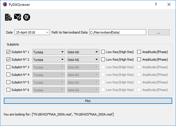
Figure 2: Select NarrowbandData folder.

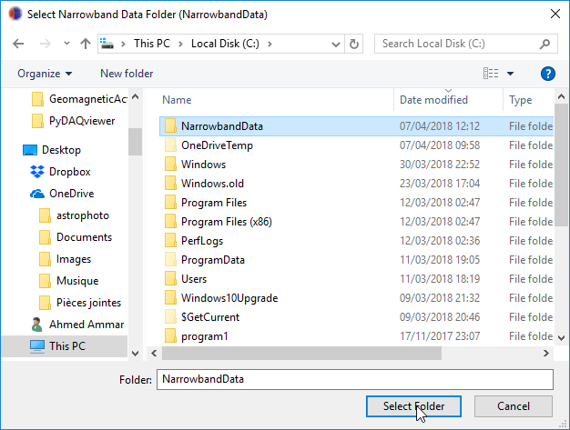
The path to your data will be something like: 'C:/NarrowbandData/SiteName/Year/MM/DD/' (e.g. 'C:/NarrowbandData/Tunisia/2018/03/25/'). Note that this can be on any drive root drive: C-Z including DVD drives etc. So if you burn data to a DVD burn it in the same folder and the PyDAQviewer will be able to find them.

Select date from calander

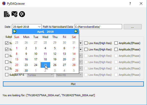
After locating the working directory, the user can select AWESOME's data recording date by using a calendar widget as shown in Figure 3.

Figure 3: Select date of the recorded data from the calendar.

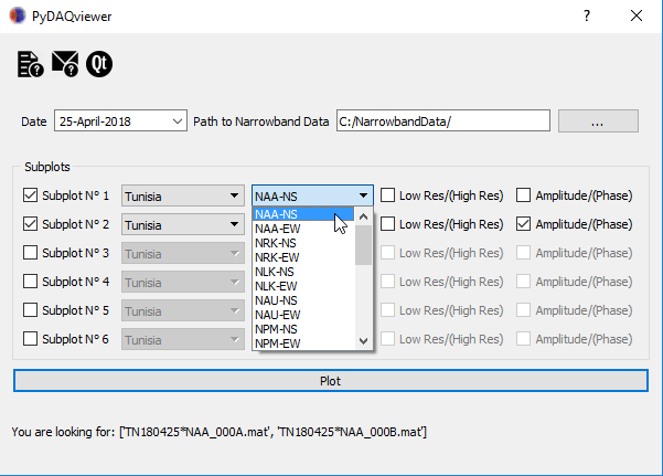
Receiver-Transmitter Information

This file is simply a Python file (Source code below: SiteInfo.py) in which you will enter two dictionaries. The first one is Rx_ID indicating the AWESOME receiver locations and their IDs. The second dictionary is Tx_ID indicating the VLF transmitter IDs and the orientation of their antennas (e.g. 000 for N/S or 001 for E/W). In this way, it is very easy to add any other receiver and transmitter IDs. Then you can simply select the Rx_ID and Tx_ID of interest via menus as shown in Figures 4 and 5.

# -*- coding: utf-8 -*-
#SiteInfo.py
'''
Purpose: Save VLF Receivers (Rx) and Transmitters (Tx) Info   
'''
# Rx info
Rx_ID = {
            "Tunisia":"TN",
            "Algeria":"AL",
            "France":"FR",
            "Japan":"JP",
            "NewYork":"NY",
            "Boulder":"BO",
            "Cheyenne":"CH",
            "Walsenburg":"WS",
            "LasVegas":"LV",
            
            
            }

# Tx info
Tx_ID = {
            "NAA-NS":"NAA_000", 
            "NAA-EW":"NAA_001",
            "NRK-NS":"NRK_000",
            "NRK-EW":"NRK_001",
            "NLK-NS":"NLK_000",
            "NLK-EW":"NLK_001",
            "NAU-NS":"NAU_000",
            "NAU-EW":"NAU_001",
            "NPM-NS":"NPM_000",
            "NPM-EW":"NPM_001",
            "ICV-NS":"ICV_000",
            "ICV-EW":"ICV_001",
            "NSC-NS":"NSC_000",
            "NSC-EW":"NSC_001",
            "GQD-NS":"GQD_000",
            "GQD-EW":"GQD_001",
            "GBZ-NS":"GBZ_000",
            "GBZ-EW":"GBZ_001",
            "DHO-NS":"DHO_000",
            "DHO-EW":"DHO_001",
            "HWU-NS":"HWU_000",
            "HWU-EW":"HWU_001",
            "JXN-NS":"JXN_000",
            "JXN-EW":"JXN_001",
            "ISR-NS":"ISR_000",
            "ISR-EW":"ISR_001"
            }

Figure 4: Select AWESOME station.

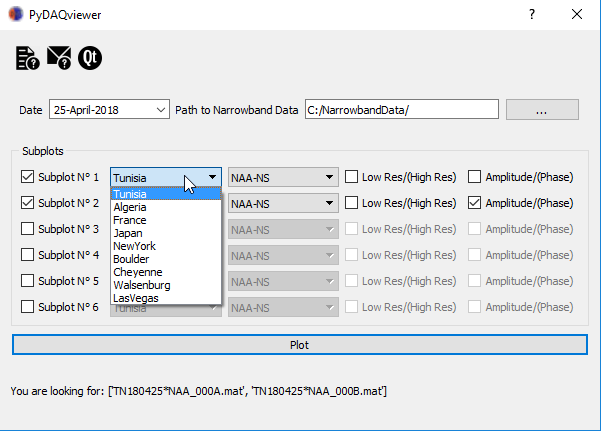
Figure 5: Select VLF transmitter.

Reproducing the Lightning-Induced Electron Precipitation (LEP) Tutorial

Now that you have a basic understanding of how the DAQviewer works, it's time to put it to the test and try out all the features. To do this we'll be reproducing a few of the plots you made by hand in the LEP tutorial.

To start edit the SiteInfo.py file to include the Rx_IDs: Cheyenne, Boulder, Walsenburg, and Las Vegas (note in the SiteInfo.py file Las Vegas should be all one word: LasVegas).

Figure 6: Example working on data from LEP tutorial.

The output of this configuration is in below:

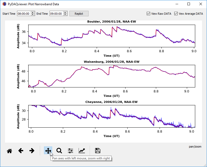
Figure 7: Generated figure.

Figure 8: Zoomed figure.